Summary of each lecture and homework/reading assignments are posted on this page after each lecture. Students are encouraged to check this page regularly.
Some useful links:
- WeBWork: Online homework
- Piazza: Discussion page for our course
- Geogebra: Contains useful tools that I picked for graphing 3D-graphs
Contents
Lecture 1
Points in Space, Coordinate Systems
Lecture Summary: In this lecture we have seen how one can describe the location of points in 3 dimensional space, which we denoted by $\mathbb{R}^3$. We have seen 3 representations:
- Rectengular coordinates: These are the standard coordinates $(x,y,z)$ of a point. You first find $(x,y)$ on the (horizontal) $xy$-plane, and then lift it up/down $z$ units, to reach the point $(x,y,z)$. That’s why the last coordinate ($z$) can be interpreted as the altitude of the point $(x,y,z)$.
- Cylindrical coordinates: If you are given a point in rectangular coordinates $(x,y,z)$, it is is easy to find its so-called cylindrical coordinates: First, look at $(x,y)$, and find its polar coordinates $(r,\theta)$. (Recall that $r=\sqrt{x^2+y^2}$ is the distance to the origin, and $\theta$ is the angle that the line segment joining the origin makes with the positive $x$-axis). Then, the cylindrical coordinates of $(x,y,z)$ is -by definition- $(r,\theta,z)$. Note that the last coordinate remains the same.
- Spherical coordinates: If you are given a point in rectangular coordinates $(x,y,z)$, its spherical coordinates are $(\rho, \theta, \varphi)$, where $\rho=\sqrt{x^2+y^2+z^2}$ is the distance to the origin, $\theta$ is as above, and $\varphi$ is the angle that the line segment joining the origin makes with the $z$-axis.
Next lecture we will see why these special coordinates are so useful in mathematics (as well as in physics and engineering).
Reading assignment: Whitman Calculus, Section 12.1, Section 12.6
Supplementary reading assignment: OpenStax Calculus 3, Section 2.7
Sample Questions for Lecture 1
Homework:
| Section 12.1: | 1, 2, 3, 6, 8-12, 16 |
| Section 12.6: | 1, 2, 4, 10 |
Lecture 2
Vectors in Space, Dot Product, Cross Product
Lecture Summary: Today we have seen the definition of a vector in $\mathbb R^2$ and $\mathbb R^3$. Essentially, a vector is an arrow that describes a displacement. A vector $\vec v$ with components $\vec v = \langle a,b,c\rangle$ describes a displacement of $a$ units in $x$-direction, $b$ units in $y$-direction, and $c$ units in $z$-direction. Vectors can be shawn as arrows, and two arrows having the same direction and length stands for the same vector. The length of a vector can be computed as $\|\vec v\|= \sqrt{a^2+b^2+c^2}$. Its direction vector is $\mathrm{dir} (\vec v) = \frac{1}{\|v\|} \vec v$. Direction vectors are always unit vectors, meaning they always have length 1.
We have also seen the dot product and cross product of vectors. If $\vec v=\langle v_1,v_2,v_3\rangle$ and $\vec w=\langle w_1,w_2,w_3\rangle$, then we define:
dot product: $\vec v\cdot\vec w = v_1 w_1 +v_2 w_2 + v_3 w_3$
cross product: $\vec v\times \vec w = \Big\langle v_2 w_3-w_2 v_3 \quad, \quad-(v_1 w_3 -w_1 v_3)\quad,\quad v_1 w_2 – w_1 v_2 \Big\rangle $
As you see, dot product is a scalar product, meaning the result will be a number. The cross product of two vectors, however, is a vector product, that is, the result will be a vector.
Next class we will study the properties of these two products, and see why they are important to study.
We have also discussed spheres and cylinders in $\mathbb R^3$. As a recap,
- The points $(x,y,z)$ satisfying $x^2+y^2+z^2=R^2$ are the points on the sphere of radius $R$ centered at the origin. In spherical coordinates, such a sphere can be expressed much easily as $\rho=R$, because $\rho$ is the distance of a point to the origin.
- The points $(x,y,z)$ satisfying $x^2+y^2=R^2$ are the points on the cylinder of radius $R$ centered at the origin. In cylindrical coordinates, this cylinder can be expressed much easily as $r=R$. Note that in $\mathbb R^2$, this is just the circle equation on the $xy$-plane. But in $\mathbb R^3$, we have the liberty of moving this circle up and down, because the equation has no “$z$” in it.
Sample Questions for Lecture 2
Reading assignment: Whitman Calculus, Section 12.2, Section 12.3, Section 12.4
Supplementary reading assignment: OpenStax Calculus 3, Section 2.1, Section 2.2, Section 2.3, Section 2.4
Homework:
| Section 12.2: | 1, 3, 6, 7, 11 |
| Section 12.3: | 1-5 |
| Section 12.4: | 1-4 |
Lecture 3
Dot-Cross Products, Ctd. & Planes in $\mathbb R^3$
Lecture Summary: Today we have started with the geometric meaning of the dot product and the cross product. Let $\vec v = \langle v_1, v_2, v_3\rangle$ and $\vec w =\langle w_1,w_2,w_3\rangle$ be two vectors in $\mathbb R^3$. Let $\theta$ be the angle between these two vectors. This means, if we think of these vectors as arrows emminating from one point, then the angle $\theta$ is the angle formed by these two arrows. Here are some useful geometric facts:
- $\vec v\cdot\vec w = \|\vec v\| \ \|\vec w\|\ \cos \theta$. This formula can be used to compute $\cos\theta = \displaystyle\frac{\vec v\cdot \vec w}{\|\vec v\|\ \|\vec w\|}$, or even $\theta = \arccos\Big(\displaystyle\frac{\vec v\cdot \vec w}{\|\vec v\|\ \|\vec w\|}\Big)$
As a consequence, if $\vec v \perp \vec w$ (meaning $\vec v$ and $\vec w$ are perpendicular (making right angle), we have $\vec v\cdot\vec w= 0,$ because $\cos\theta=\cos 90^\circ = 0$. - $\|\vec v\times\vec w\| = \|\vec v\| \ \|\vec w\|\ \sin \theta$. As above, this can be used to compute $\sin \theta$ and $\theta$, too!
As a consequence, we have $\vec v \times \vec v = \langle 0,0,0\rangle$ (the zero vector), because the angle between $\vec v$ and itself is $\theta =0$, and we have $\sin 0=0$. - We have also seen the right hand rule, which is used to determine the direction of $\vec v\times\vec w$ by looking at the directions of $\vec v$ and $\vec w$. You need stretch your 4 fingers of your right hand toward $\vec v$, and curl them towards $\vec w$. Then, your thumb will point towards $\vec v\times\vec w$. Note that $\vec v\times\vec w$ is always perpendicular to $\vec v$ and $\vec w$, and hence, it is perpendicular to the plane containing $\vec v$ and $\vec w$.
- $\vec v \cdot \vec w=\vec w\cdot \vec v$
$\vec v \times \vec w=-\vec w\times \vec v$
We have also started talking about planes in $\mathb R^3$. We have derived the following formulation:
Equation of a plane: If $P=(x_0,y_0,z_0)$ is a point on the plane, and if $\vec n = \langle a,b,c\rangle$ is a normal vector (a perpendicular vector) to the plane, then any point $(x,y,z)$ on the plane must obey the following rule:
$a(x-x_0)+b(y-y_0)+c(z-z_0)=0$
This is called the equation of that plane.
Next class we will see some examples. Also, we will talk about equation of lines in 3-dimensional space, and their generalizations.
Reading assignment: Whitman Calculus, Section 12.3, Section 12.4, Section 12.5
Supplementary reading assignment: OpenStax Calculus 3, Section 2.3, Section 2.4, Section 2.5
Homework:
| Section 12.3: | 6-8,16,18 |
| Section 12.4: | 5,8,9 |
| Section 12.5: | 1-4 |
Lecture 4
Line equations & Vector valued functions
Lecture Summary: Today we discussed how one describes a straight line in three dimensional space $\mathbb R^3$. To describe a line $L$ we need
- A point $P=(x_0,y_0,z_0)$ on the line
- A direction vector $m=\langle a,b,c\rangle$, which is parallel to the line.
In that case, the line is described mathematically by THREE equations:
$x=x_0 + at$
$y=y_0 + bt$
$z=z_0+ct $
or for short
$\vec r(t)=\langle x_0 + at, y_0 + bt, z_0+ct\rangle$.
An example that we discussed involved finding the line of intersection of two planes. Here, the crucial point was to find a direction vector $\vec m$ of this line. We noted that such a vector must lie on both planes (being on the line of intersection), and thus, must be perpendicular to normal vectors $\vec n_1$ and $\vec n_2$ of the planes. Hence, $\vec m\perp \vec n_1$ and $\vec m\perp \vec n_2$. So we can tak $\vec m =\vec n_1\times \vec n_2$.
Towards the end of the lecture we started talking about vector valued functions. These are functions with three components, given of the form
$\vec r(t)=\langle f(t),g(t),h(t)\rangle$.
Vector valued functions have graphs, because they indicate the position of a point at time $t$. As an example we saw:
- $\vec r(t)=\langle \cos t ,\sin t, 0\rangle$ is the unit circle on the $xy$-plane; the initial point $\vec r(0)$ is the point $(1,0,0)$ on the $x$-axis, and the movement is in the counterclockwise direction when observed from above the $xy$-plane
- $\vec r(t)=\langle \sin t ,\cos t, 0\rangle$ is also the unit circle on the $xy$-plane, but the initial point $\vec r(0)=\langle 0,1,0\rangle$ is on the $y$-axis, and the rotation is in clockwise direction.
- $\vec r(t)=\langle \cos t ,\sin t, t\rangle$ is the helix where the movement is upwards and counterclockwise as time increases.
In general these graphs are difficult to sketch by hand, so we are not going to sketch them. Rather we are going to make calculations with them (next class). If you absolutely want to see the graph, you can use the “parametrized curve sketching” took in Geogebra (the link is on the opt of this page).
Reading assignment: Whitman Calculus, Section 12.5, Section 13.1
Supplementary reading assignment: OpenStax Calculus 3, Section 3.1, Section 3.2, Section 3.3
Homework:
| Section 12.5: | 5-10 |
| Section 13.1: | 1-4 (use the Sage code in the exercise section) |
Lecture 5
Tangent lines, Multivariable Functions
Lecture Summary: Today we started with an important observation. Given a vector valued function $\vec r(t)=\langle f(t),g(t),h(t) \rangle$, it gives the position of a point moving in space. Its derivative $\vec r'(t)=\langle f'(t),g'(t),h'(t)\rangle$ represents the velocity vector, which indicates the direction of movement at every point of $\vec r(t)$. As a consequence, $\vec r'(t)$ is a tangent vector to the curve at the point $\vec r(t)$. In particular, it is the in the direction of the tangent line at that point. So you can use $\vec r'(t)$ as the direction vector $\vec m$ that we talked about in the previous lecture.
Another important thing we learned was how to compute the length of a curve (sometimes called arclength). Let $\vec r(t)=\langle f(t),g(t),h(t) \rangle$ be a given curve where the time parameter is bounded from $a$ to $b$ (such a bound is necessary as we don’t want to compute the length of an unbounded curve because it would just be $\infty$). Then, the length of this curve is given by the integral of the speed:
$$\int_a^b \|\vec r'(t)\| \ dt=\int_a^b \sqrt{[f'(t)]^2+[g'(t)]^2+[h'(t)]^2} \ dt.$$
This integral may be tedious, because we have a square-root under an integral, and square-roots and intgrals don’t get along well. Most of the integrals you will see in this course, however, will be easy to compute. You may have to simplify the square-root expression first before attempting the integration.
We have also seen examples of several surfaces:
$z=5$ (horizontal plane 5 units above the $xy$-plane)
$z=x^2+y^2$ (paraboloid)
$z=-x^2-y^2$ (upside down paraboloid)
$z=\sqrt{x^2+y^2}$ (upper cone)
$z=-\sqrt{x^2+y^2}$ (lower cone)
$z=\sqrt{9-x^2-y^2}$ (upper semisphere of radius 3 with center at origin)
$z=-\sqrt{9-x^2-y^2}$ (lower semisphere of radius 3 with center at origin)
Sample Questions (TBA)
Reading assignment: Whitman Calculus, Section 13.2, Section 13.3
Supplementary reading assignment: OpenStax Calculus 3, Section 4.1, Section 2.6
Homework:
| Section 13.2: | 1-5 |
| Section 13.3: | 1-5 |
Lecture 6
Level Curves, Partial Derivatives
Lecture Summary: In this lecture we discussed the notion of level curves. Given a function $z=f(x,y)$. Its graph is a surface in space (see examples in the previous lecture. Now, imagine you cut this surface horizontally with a horizontal plane $z=c$. The intersection will be some curve. All points on this curve will have the $z$-coordinate $c$. Therefore, the curve will satisfy $c=f(x,y)$. It is called the level-$c$ curve of the function $z=f(x,y)$.
We have also seen the concept of partial derivatives. Consider a function $f(x,y)$. Then we have two notions of derivative:
- Treat $y$ as a constant, and take the derivative of $f(x,y)$ with respect to $x$. You get the partial derivative with respect to $x$, which is denoted by $\displaystyle\frac{\partial f}{\partial x}=f_x$.
- Treat $x$ as a constant, and take the derivative of $f(x,y)$ with respect to $x$. You get the partial derivative with respect to $y$, which is denoted by $\displaystyle\frac{\partial f}{\partial y}=f_y$.
Next class we will see applications of these concepts.
Sample Questions (TBA)
Reading assignment: Whitman Calculus, Section 14.1, Section 14.3, Section 14.6
Supplementary reading assignment: OpenStax Calculus 3, Section 4.3, Section 4.4
Homework:
| Section 14.1: | 6 |
| Section 14.3: | 1-7 |
| Section 14.6: | 1-7 |
Lecture 7
Tangent Planes, Normal Lines, Chain Rule
Lecture Summary: In this lecture we have seen applications of partial derivatives. Supposed that we have a function (for example, the cost of a certain product that depends on many ingredients/parts), let’s call it $f(x,y,z,t,…)$. Partial derivative of this function $f$ with respect to a variable, say $x$, is obtained by fixing all the other variables, and looking at how the value of $f$ changes only when $x$ changes. In economics and law, this idea is called ceteris paribus (in latin, ceterus=other as in et cetera, and par=even/equal/comparable, both words in ablative/dative plural form), meaning keeping all the other things the same.
We have seen that a normal vector to a given surface can be computed using partial derivatives. Indeed:
- If the surface is given in the explicit form $z=f(x,y)$, a normal vector to the surface at a point $(x,y,f(x,y))$ is given by $$\vec n =\langle -f_x, -f_y, 1\rangle.$$
- If the surface is given in the implicit form $F(x,y,z)=0$, a normal vector to the surface at a point $(x,y,z)$ is given by $$\vec n =\langle F_x, F_y, F_z\rangle.$$
Once you find the normal vector to the surface, you can write down the equation of the tangent plane to the surface at that point, because the same normal vector will be perpendicular to the tangent plane as well.
Also, note that once you know one normal vector, you know all the other normal vectors at that point, because all normal vectors at one particular point are parallel.
We also talked about normal line which is the line perpendicular to the surface, in the direction of the normal vector.
Towards the end of the lecture, we discussed the chain rule in multivariable calculus. We developed the idea of tree of dependence among the variables in your function, and we derived various chain rule formula using these trees.
To summarize:
Chain rule in single variable calculus: Given a function $y=f(x)$ and assume that $x=g(t)$. Then $y$ becomes $y=f(g(t))$, essentially making it depend on $t$. Hence, we can think about the rate of change (derivative) of $y$ with respect to $t$. This derivative is related to the derivative of $y$ with respect to $x$, and is given by the chain rule formula: $$\displaystyle \frac{dy}{dt} = \frac{dy}{dx}\cdot \frac{dx}{dt}$$
Chain rule in multivariable calculus: Given a function $z=f(x,y)$, and assume that $x=g(t)$ and $y=h(t)$. Then $z$ becomes $z=f(g(t),h(t))$, essentially making it depend on $t$. Now we can compute the derivative of $z$ with respect to $t$ using the following multivariable chain rule formula: $$\displaystyle \frac{dz}{dt} = \frac{\partial z}{\partial x}\cdot \frac{dx}{dt} + \frac{\partial z}{\partial y}\cdot \frac{dy}{dt}$$
We will talk more about this next lecture.
Sample Questions (TBA)
Reading assignment: Whitman Calculus, Section 14.3, Section 14.4
Supplementary reading assignment: OpenStax Calculus 3, Section 4.3, Section 4.4, Section 4.5
Homework:
| Section 14.3: | 8-12 |
| Section 14.4: | 1-6 |
Lecture 8
Test 1
Comments about the test: TBA
Lecture 9
Chain Rule, Gradient, Directional Derivatives
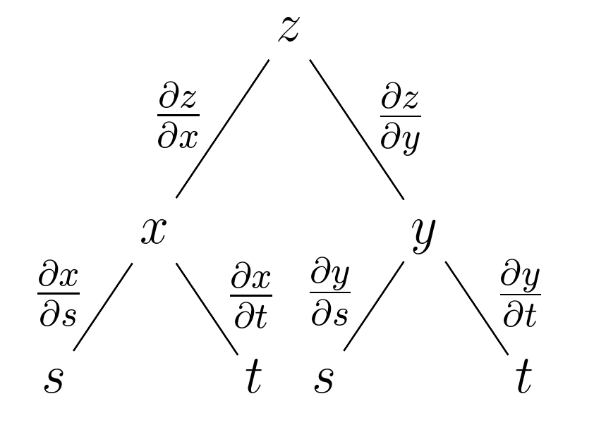
Lecture Summary: We started with a review of chain rule which we had studied earlier. The key idea is to sketch a tree of dependency. For instance, if we are given a function $z=f(x,y)$ where $x=g(s,t)$ and $y=h(s,t)$, then we have the following dependency tree:
 From here we have the following chain rules:
$$\displaystyle \frac{\partial z}{\partial t} = \frac{\partial z}{\partial x}\cdot \frac{\partial x}{\partial t} + \frac{\partial z}{\partial y}\cdot \frac{\partial y}{\partial t}$$
$$\displaystyle \frac{\partial z}{\partial s} = \frac{\partial z}{\partial x}\cdot \frac{\partial x}{\partial s} + \frac{\partial z}{\partial y}\cdot \frac{\partial y}{\partial s}$$
We also saw the notion of the gradient of a function $f(x,y)$. It is a vector denoted by $\nabla f$, and has partial derivatives of $f$ as its components. Namely, $$\nabla f =\langle f_x , f_y \rangle .$$ For example, if $f(x,y) =2x^2y^3+x+5y$, then $\nabla f = \langle 4xy^3+1, 6x^2 y^2 +5 \rangle$.
Gradients are used in what is known as the directional derivatives of functions. Imagine you are standing at a point $(x,y,f(x,y))$ on a surface $z=f(x,y)$, which you can think of as a mountain. Now, if you were to walk in a particular direction vector $\vec u = \langle a,b \rangle$, then the slope of the trail at the point $(x,y,f(x,y))$ is called the directional derivative of the function $f$ at point $(x,y)$ in the direction of $\vec u$. This directional derivative is denoted by $D_u f$. It is very easy to compute: $$D_u f = \nabla f\cdot \vec u = \langle f_x, f_y \rangle \cdot \langle a,b\rangle = a\ f_x + b \ f_y$$
Directional derivatives are generalization of partial derivatives. The directional derivative in the $x$-direction (namely when $\vec u = \vec i = \langle 1, 0 \rangle$) is precisely the partial derivative $f_x$. Similarly, the directional derivative in the $y$-direction (namely when $\vec u = \vec j = \langle 0,1 \rangle$) is precisely the partial derivative $f_y$.
One thing to keep in mind is that $\vec u$ is always taken as a unit vector (that is, a vector of length 1) in the context of directional derivatives. If it happens that $\vec u$ is not a unit vector, we can make it a unit vector by dividing it by its length.
We observed that, at any point, the directional derivative $D_u f = \nabla f \cdot \vec u = \| \nabla f\| \ \|\vec u \| \cos \theta $ is MAXIMUM when $\nabla f$ and $\vec u $ point in the same direction, and minimum when they point in the opposite directions. In other words, the altitude on a surface $z=f(x,y)$ increases the most in the direction of $\nabla f$ and decreases the most in the direction of $-\nabla f$. Physically, this means the following: Imagine you release a ball on a mountain (whose surface is given by the equation $z=f(x,y)$). Then, naturally, the ball will start moving because of Earth’s gravity. In which direction will the ball start rolling? Answer: in the direction $\nabla f= \langle f_x, f_y\rangle$. This is known as the gradient flow, and has many applications, in broader contexts, in mathematics, physics, and engineering.
Sample Questions (TBA)
Reading assignment: Whitman Calculus, Section 14.5
Supplementary reading assignment: OpenStax Calculus 3, Section 4.6
Homework:
| Section 14.5: | 1-7, 10-18 |
Lecture 10
Max-Min Problems
Lecture Summary: Today we started talking about max-min problems. Given a curve $y=f(x)$. At a point $x=x_0$ where there is a horizontal tangent line, we have $f'(x_0)=0$, and the graph has either a local max, a local min, or an inflection point.
- If $f”(x_0)>0$, the graph has a local minimum;
- if $f”(x_0)<0$, the graph has a local maximum;
- if $f”(x_0)=0$, but $f”(x)$ changes sign at $x_0$, there is an inflection point.
We have an analogous picture in 3D. At a local max or min, we have a horizontal tangent plane, which means that the normal vector is vertical. As a consequence we have, $f_x=0$ and $f_y =0$ (because $\vec n=\langle -f_x,- f_y, 1\rangle$).
However, there are surfaces which have horizontal tangent planes at a point which is neither local max nor a local min. These points are called saddle points. In geology, these structures are called mountain passes. In the South, especially along Appalachians, people call it mountain gaps.

Sample Questions (TBA)
Reading assignment: Whitman Calculus, Section 14.7
Supplementary reading assignment: OpenStax Calculus 3, Section 4.7
Homework: No homework for this lecture. Please read the sections from the textbook prior coming to the next class.
Lecture 11
Max-Min Problems
Lecture Summary: Today we have studied max-min problems for functions $z=f(x,y)$. First, we find the critical points. These are the points at which the graph of the function $z=f(x,y)$ has a horizontal tangent. To do this, we set $f_x$ and $f_y$ equal to zero, and solve for $(x,y)$. The solutions, which are by definition the critical points, fall into three categories. They are either a local max, local min, or a saddle point. The find out which, we apply the second derivative test.
The second derivative test involves computing a quantity $$D=\det \left(\begin{array}{cc} f_{xx} & f_{xy}\\ f_{yx} &f_{yy} \end{array}\right) = f_{xx}\ f_{yy} – (f_{xy})^2.$$
Let $(x_0,y_0)$ be a critical point. Then we conclude:
- If $D>0$ and $f_{xx}>0$ at $(x_0,y_0)$, then $(x_0,y_0)$ is a local minimum
- If $D>0$ and $f_{xx}<0$ at $(x_0,y_0)$, then $(x_0,y_0)$ is a local maximum
- If $D<0$ at $(x_0,y_0)$, then $(x_0,y_0)$ is a saddle point.
- If $D=0$, use another method to figure out what kind of a point $(x_0,y_0)$ is.
As an application, we have considered a concrete problem. Let’s say we have a 20 inch wire, and we cut it in three pieces. Using the first piece, we construct a square, using the second we construct a rectange with ratio 2:1, and using the third we construct an equilateral triangle. How should we cut the wire so we get the minimum area.
The problem was fully solved in class. I have developed a graphic application which we can use to verify thesolution of the problem visually.
Sample Questions (TBA)
Reading assignment: Whitman Calculus, Section 14.7
Supplementary reading assignment: OpenStax Calculus 3, Section 4.7
Homework:
| Section 14.7: | 1-6 |
Lecture 12
Lagrange Multipliers
Lecture Summary: Last time we had seen how to find maximum/minumum values of a function $f(x,y)$ when $(x,y)$ belongs to the domain of $f(x,y)$ (usually on whole of $xy$-plane $\mathbb R^2$). Physically/Geometrically, this corresponds to finding the points of highest/lowest altitude of a surface $z=f(x,y)$, for example if we see it as a mountain.
Today we have seen a different type of optimization problem: How to find maximum and minimum of a function $f(x,y)$ when $(x,y)$ belongs to a curve $g(x,y)=d$ on the $xy$-plane.
Physically/Geometrically this corresponds to finding the points of highest/lowest altitude on a path on the mountain $z=f(x,y)$. This path is the one that is obtained by lifting the curve $g(x,y)=d$ to the surface.
We have seen that at a point of maximum/minimum on this path, two equations must hold:
- $\nabla f = \lambda \nabla g$. In other words, the gradients of $f$ and $g$ must align.
- $g(x,y)=d$. In other words, the point must be on the path on the mountain.
These two equations will form a non-linear (and non-standard) system of equations, which can be solved for $x$,$y$,$\lambda$ by a careful analysis. We have seen a lot of examples where we had to consider different cases depending on the values of $x$,$y$,$\lambda$.
Sample Questions (TBA)
Reading assignment: Whitman Calculus, Section 14.8
Supplementary reading assignment: OpenStax Calculus 3, Section 4.8
Homework:
| Section 14.8: | 13, 14 |
Lecture 13
Regions on xy-plane, Double integrals
Lecture Summary: Today we have seen how one can describe certain regions on $xy$-plane mathematically. We have concentrated on two categories of examples:
- TYPE-1 REGIONS: These are regions of the form $$\{(x,y): a\leq x\leq b,\ g(x)\leq y\leq h(x) \}.$$ Geometrically, this means, as $x$ runs from $a$ to $b$, we scan the region using vertical lines going from the curve $y=g(x)$ to $y=h(x)$.
- TYPE-2 REGIONS: These are regions of the form $$\{(x,y): c\leq y\leq d,\ g(y)\leq x\leq h(y) \}.$$ Geometrically, this means, as $y$ runs from $c$ to $d$, we scan the region using horizontal lines going from the curve $x=g(y)$ to $x=h(y)$.
After that, we have defined a notion of integral for multivariable functions $z=f(x,y)$. Specifically, if $D$ is a region on $xy$-plane, then we define the double integral of $f(x,y)$ over $D$ as $$\displaystyle \iint\limits_D f(x,y) dA$$ to be the (signed) volume between the graph of $z=f(x,y)$ and the region $D$ on the $xy$-plane. Signed volume is the same as the regular volume, except that if the surface lies below the $xy$-plane somewhere, the volume between the surface and the $xy$-plane over there is counted as negative. (This should remind you of the geometric interpretation of single integrals).
At the end of the class we have seen a very fundamental theorem, called Fubini’s theorem, which helps us compute the double integrals over type-1 or type-2 regions.
Fubini’s Theorem:
- If $D=\{(x,y): a\leq x\leq b,\ g(x)\leq y\leq h(x) \}$ is a type-1 region, then $$\displaystyle \iint\limits_D f(x,y) dA = \int_a^b \left( \int_{g(x)}^{h(x)} f(x,y) dy \right) dx.$$
- If $D=\{(x,y): c\leq y\leq d,\ g(y)\leq x\leq h(y) \}$ is a type-2 region, then $$\displaystyle \iint\limits_D f(x,y) dA = \int_c^d \left( \int_{g(y)}^{h(y)} f(x,y) dx \right) dy$$
Note that first we compute the inner integrals (inside the parentheses), and then we compute the outer integral. Pay attention to the variable with respect to which you are integrating. That’s why the symbols $dx$ and $dy$ play a crucial role in double integrals. This should remind you of the integrals in washer and shell methods in Calculus 2.
Next lecture will be devoted to examples.
Sample Questions (TBA)
Reading assignment: OpenStax Calculus 3, Section 5.2
Homework: No homework for this lecture. Just complete the reading assignment.
Lecture 14
Double integrals, continued
Lecture Summary: Today we have seen more examples and applications of double integrals.
Sample Questions (TBA)
Reading assignment: OpenStax Calculus 3, Section 5.2
Supplementary reading assignment: Whitman Calculus, Section 15.1
Homework:
| Section 15.1: | 1-8, 16 |
| Section 5.2: | page 520: 60, 63, 68, 71, 74, 75, 80, 85, 100, 101 |
Lecture 15
Review
Lecture Summary: We had a review for the upcoming test.
Lecture 16
Test 2
Comments about the test:
Lecture 17
Triple Integrals, Polar Regions
Lecture Summary: Today we started with generalizing the double integral to one dimension higher, to get what is called triple integral. Recall that a typical double integral is $$\displaystyle\iint\limits_{D} f(x,y) \ dA$$ is the integral of a function of TWO variables over a region $D$ in the TWO-dimensional xy-plane. If $D$ is, say, a type-1 region, we can convert this double integral into two single integral. That is, if $D=\{(x,y): a\leq x\leq b,\ g(x)\leq y\leq h(x) \}$ then we have $$\displaystyle \iint\limits_D f(x,y) dA = \int_a^b \left( \int_{g(x)}^{h(x)} f(x,y) dy \right) dx.$$ To generalize this to one dimension higher, we should consider TRIPLE integrals of functions $f(x,y,z)$ of THREE variables over a solid $U$ in the THREE-dimensional $xyz$-space. The notation for this integral will be $$\displaystyle\iiint\limits_{U} f(x,y,z) \ dV$$ which can be computed by $$\displaystyle \iiint\limits_U f(x,y,z) \ dV = \int_{x=a}^b \int_{y=g(x)}^{h(x)} \int_{z=k(x,y)}^{m(x,y)} dz \ dy\ dx.$$ if the solid $U$ is given as $U=\{ a\leq x\leq b, \ g(x)\leq y\leq h(x), \ k(x,y)\leq z \leq m(x,y) \}$.
Next we looked at polar regions. These are regions described by the polar coordinates $r$ and $\theta$.
Sample Questions (TBA)
Reading assignment: Whitman Calculus, Section 15.5
Supplementary reading assignment: OpenStax Calculus 3, Section 5.4
Homework:
| Section 15.5: | 1,2,10 |
Lecture 18
Integration on Polar regions
Lecture Summary: If a region in $\mathbb R^2$ is given in terms of polar coordinates such as $$D=\{ \alpha\leq\theta\leq \beta, \ g(\theta)\leq r\leq h(\theta) \},$$ then we can compute the double integral of any function $f(x,y)$ as follows. $$\displaystyle \iint\limits_{D} f(x,y) \ dA = \int_{\theta=\alpha}^{\beta} \int_{r=g(\theta)}^{h(\theta)} f(r\cos\theta, r\sin\theta) \ r\ dr\ d\theta.$$
The crucial point here is that $x$ gets replaced by $r\cos\theta$, $y$ by $r\sin\theta$, AND $dA$ by $r\ dr\ d\theta$. The extra $r$ is very important, we will see later where it comes from.
Sample Questions (TBA)
Reading assignment: Whitman Calculus, Section 15.2
Supplementary reading assignment: OpenStax Calculus 3, Section 5.3
Homework:
| Section 15.2: | 8,12,13 |
| Section 5.3: | p.540: 122-132,135,157, |
Lecture 19
Vector Fields
Lecture Summary: Today we have studied vector fields. Roughly speaking, a vector field is a vector with variable components. Examples would be
| $\langle x+y, x^2-y^2\rangle$ | A vector field in $\mathbb R^2$ |
| $\langle 2xz+5y, 3yz, x+1\rangle$ | A vector field in $\mathbb R^3$ |
To sketch vector fields you can use the graphing tools on Geogebra, for example this one for 2D-vector fields, and this for 3D-vector fields.
Typical examples of vector fields are gradient of functions: $\nabla f$. Such vector fields are called conservative vector fields.
We have seen that a vector field $\langle P,Q\rangle$ defined on all of $\mathbb R^2$ is a conservative vector field if the equality $$Q_x = P_y$$ holds everywhere.
Next class we will see a 3D-version of this theorem. Namely, when is a vector field $\langle P,Q,R\rangle$ in $\mathbb R^3$ is conservative (that is, gradient of a function)? The result is very interesting, and quite complicated.
Sample Questions (TBA)
Reading assignment: Whitman Calculus, Section 16.1
Supplementary reading assignment: OpenStax Calculus 3, Section 6.1
Homework:
| Section 16.1: | 1-6 (use the sage code to sketch the vector fields) |
Lecture 20
Line Integral of functions
Lecture Summary: Today we have started with conservative vector fields in $\mathbb R^3$.
Given a vector field $\vec F=\langle P,Q,R\rangle$ in $\mathbb R^3$. If the vector field $$curl \vec F = \langle R_y-Q_z, P_z-R_x, Q_x-P_y\rangle$$ is identically $0$, then it turns out that the vector field is conservative (that is, it is the gradient $\nabla f = \langle f_x,f_y,f_z\rangle$ for some function $f(x,y,z)$.
Next, we studied line integrals of functions in $\mathbb R^2$ and $\mathbb R^3$.
Let $C$ be a curve from a point $A$ to $B$ in $\mathbb R^2$ or $\mathbb R^3$. Let $\vec r(t)$ be a parametrization for $C$, where $a\leq t\leq b$. That is, $\vec r(a)=A$ and $\vec r(b)=B$, and $\vec r(t)$ runs over the curve $C$ as $t$ runs from $a$ to $b$. In this case, we define the line integral of a function $f$ on $\mathbb R^2$ or $\mathbb R^3$ by $$\displaystyle \int\limits_C f \ ds = \int_a^b f(\vec r(t))\ \|\vec r\ ‘(t)\| \ dt.$$
Next time we will see lots of examples. We will also see how to integrate vector fields over curves.
Sample Questions (TBA)
Reading assignment: Whitman Calculus, Section 16.2
Supplementary reading assignment: OpenStax Calculus 3, Section 6.1, Section 6.2
Homework:
| Section 16.2: | 1-3 |
| Section 6.1 | p.660 26, p.708 106-111, 116-123 |
Lecture 21
Line integral of vector fields
Lecture Summary: Today we studid line integrals of vector fields. Let $\vec F=\langle P,Q,R\rangle $ be a vector field in $\mathbb R^3$. Let $C$ be an (oriented) curve in $\mathbb R^3$ parametrized by $\vec r(t)$, where $a\leq t\leq b$. Then we define the line integral of a function $f(x,y,z)$ over $C$ as $$\int\limits_C \vec F \cdot d\vec r = \int_{a}^b \vec F(\vec r(t)) \cdot \vec r\ ‘(t) \ dt.$$ There is an alternative notation for these type of integrals: $$\int\limits_C \vec F \cdot d\vec r =\int\limits_C \langle P,Q,R \rangle\cdot d\vec r = \int\limits_C \langle P,Q, R\rangle\cdot \langle dx,dy,dz\rangle = \int\limits_C P\ dx +Q\ dy + R \ dz.$$
If the vector field $\vec F$ is conservative, that is, if $F=\nabla f$, then the line integrals are extremely easy to integrate. Let $C$ be any curve from point $A$ to point $B$. Then $$\int\limits_C \vec F \cdot d\vec r =\int\limits_C \nabla f \cdot d\vec r = f(B)-f(A).$$
In particular, the line integrals of vector fields depend only on the endpoints of the curve $C$, not on the actual trail of the curve. For example, if $C$ is a closed curve, meaning the initial and terminal points are the same, then the line integral of a conservative vector field is always zero.
Note that the line integral of a non-conservative vector field over closed curve may not be zero.
Sample Questions (TBA)
Reading assignment: Whitman Calculus, Section 16.2, Section 16.3
Supplementary reading assignment: OpenStax Calculus 3, Section 6.2, Section 6.3
Homework:
| Section 16.2: | 4-14 |
| Section 16.3: | 1-11 |
Lecture 22
Green’s Theorem
Lecture Summary: Today we have seen one of the cornerstone results of this course: The Green’s Theorem.
Let $C$ be a closed curve in the plane $\mathbb R^2$. Roughly speaking, this means, the curve starts and ends at the same point. Closed curves always enclose a region $R$. An orientation is simply a directional arrow on $C$. We say that $C$ is positively oriented if our left hand points towards $R$ as we walk along $C$.
| Green’s Theorem: Let $C$ be a positively oriented closed curve enclosing a region $R$. Let $\vec F= \langle P,Q \rangle$ be a vector field in $\mathbb R^2$. Then $$\displaystyle \int\limits_C \vec F\cdot d\vec r = \iint\limits_R Q_x -P_y \ dA.$$ |
In particular, if $\vec F=\nabla f$ is conservative, that is, if $Q_x=P_y$, then $\displaystyle\int_C \nabla f\cdot d\vec r = 0$, as we also observed in the previous class.
We have seen some examples today indicating the power of Green’s theorem for line integrals over closed curves.
Next lecture will be a comprehensive review for the test.
Sample Questions (TBA)
Reading assignment: Whitman Calculus, Section 16.4
Supplementary reading assignment: OpenStax Calculus 3, Section 6.4
Homework:
| Section 16.4: | 1-13 |
| Section 6.4: | p.733: 146, 147, 155, 158, 159, 181 |
Lecture 23
Review
Lecture Summary: Today we have reviewed the material for the test. Basically, there are 5 topics:
- Double integrals over polar coordinates
- Triple integrals
- Vector fields (including conservative vector fields, and how to find their potentials)
- Line integrals (both of the form $\displaystyle \int\limits_C f(x,y,z) \ ds$ and $\displaystyle\int\limits_C \vec F \cdot d\vec r$.
- Green’s Theorem (which we use to compute $\displaystyle\int\limits_C \vec F \cdot d\vec r$ in case when $C$ is a closed curve).
If you have any questions about webwork, worksheets, or textbook problems, feel free to post them on Piazza over the spring break.
Lecture 24
Test 3
Comments about the test:
Lecture 25
Surface Integral
Lecture Summary: As the final piece of the puzzle of multivariable calculus, we have seen the surface integral today. As in line integrals, we can define surface integrals of functions $f(x,y,z)$ and vector fields $\vec F(x,y,z) = \langle P,Q,R \rangle$.
Regardless if it is a function or a vector field we are integrating, the surface integrals are always defined on a surface. For convenience, in this course we will only consider surfaces $S$ of the form $z=g(x,y)$. Note that points on such a surface are given as $(x,y,g(x,y))$ where $(x,y)$ is in a domain $D$ on the $xy$-plane. Geometrically, $D$ is the shadow (projection) of the surface $S$ in $xyz$-space onto the $xy$-plane.
In this setting, the surface integrals are defined as follows:
- The surface integral of a function $f(x,y,z)$ on the surface $S$ given by $z=g(x,y)$ (defined over the region $D$ on the $xy$-plane) is defined by $$\displaystyle\iint\limits_{S} f(x,y,z) \ dS = \iint\limits_{D} f(x,y,g(x,y)) \|\langle -g_x, -g_y , 1 \rangle\| \ dA$$.
- The surface integral of a vector field $\vec F(x,y,z)$ on the upward oriented surface $S$ given by $z=g(x,y)$ (defined over the region $D$ on the $xy$-plane) is defined by $$\displaystyle\iint\limits_{S} \vec F(x,y,z)\cdot \ d\vec S = \iint\limits_{D} \vec F (x,y,g(x,y)) \cdot \langle -g_x, -g_y , 1 \rangle \ dA$$.
Observe that the term $\langle -g_x, -g_y , 1 \rangle $ in these integrals is just a normal vector field to the surface $z=g(x,y)$. It is known as the upward pointing normal vector. If we consider the negative of this vector field we get $\langle g_x, g_y ,- 1 \rangle $ which is called the downward normal. The question must specify which normal vector field we should use in the integration. If not, just use the upward pointing one. The answer should only differ by a negative sign.
Note that in each case we convert the given surface integral $$\displaystyle\iint\limits_S \cdots$$ into a double integral $$\displaystyle\iint\limits_D \cdots dA$$.
Since we already know how to compute double integrals (by determining whether $D$ is a type 1/2 or polar region), we can compute the surface integrals.
Because of the extra step of conversion into a double integral, surface integrals take more time to compute than plain double integrals. But, they are used a lot in physics and engineering. If $\vec F$ stands for the velocity vector field of some fluid in space, then the surface integral of $\vec F$ computes the flux of the fluid through the surface, that is, the amount of fluid flowing through the surface.
Sample Questions (TBA)
Reading assignment: Whitman Calculus, Section 13.2
Supplementary reading assignment: OpenStax Calculus 3, Section 6.6
Homework:
| Section 16.7: | 5-9 (converting into iterated integral is enough) |
| Section 6.6: | p 784: 284, 297-300, 312 |
Lecture 26
Stokes’ Theorem
Lecture Summary: Today we have learnt one of the most important theorems in Calculus, the Stokes’ Theorem.
If $S$ is a surface in $\mathbb R^3$ we denote its boundary curve by $\partial S$. Here, $\partial$ is not the partial derivative, it is a symbol that is read as “boundary”. So, $\partial M$ is read as “boundary of $M$”. For example, if $S$ is the upper-semisphere of radius 1, centered at the origin, then $\partial S$ is the circle of radius 1 centered at the origin on the $xy$-plane.
If we are given a normal vector field for $S$, like $\langle -g_x,-g_y,1\rangle$ for the surface $z=g(x,y)$, there is an induced/compatible orientation on the boundary that is found using the right hand rule: If you point your thumb to the normal vector, your fingers will curl towards the correct orientation of the boundary.
Now, under the suitable choice of orientations, Stokes’ theorem gives us a relation between a line integral on $C=\partial S$ and a surface integral on $\partial S$.
Stokes Theorem: Let $S$ be a surface in $\mathbb R^3$ and let $C=\partial S$ be its boundary, with the induced orientation. Then $$\int\limits_C \vec F\cdot d\vec r = \iint\limits_S curl \vec F \cdot d \vec S.$$
Note that some textbooks use the notation $\nabla \times \vec F$ for $curl \vec F$, and some use $\displaystyle\iint \vec F \cdot \vec N \ dS$ for $\displaystyle\iint \vec F \cdot d\vec S $. Keep this in mind when solving problems.
Sample Questions (TBA)
Reading assignment: Whitman Calculus, Section 16.8
Supplementary reading assignment: OpenStax Calculus 3, Section 6.7
Homework:
| Section 16.8: | 2-4 (Convert to iterated integrals. You do not need to compute iterated integrals explicitly.) |
| Section 6.7: | p.802: 329, 332, 333, 339 |
Lecture 27
Gauss’ Theorem
Lecture Summary: Today we have studied Gauss’ Theorem, a.k.a. Divergence Theorem.
What is Divergence of a Vector Field? Let $\vec F = \langle P,Q,R\rangle$ be a vector field. Then, we define $div\vec F$ to be $P_x+Q_y+R_z$. Note that $div \vec F$ is a scalar, not a vector.
Gauss’ Theorem: Let $\matchcal U$ be a solid in $\mathbb R^3$ with a boundary surface $\partial \mathcal U = S$. Assume that $S$ has outward orientation. Then, $$\iint\limits_S \vec F \cdot d\vec S = \iiint\limits_{\mathcal U} div \vec F \ dV.$$
Sample Questions (TBA)
Reading assignment: Whitman Calculus, Section 16.9
Supplementary reading assignment: OpenStax Calculus 3, Section 6.8
Homework:
| Section 16.9: | 3-8 |
| Section 6.8: | p.819: 376-380 |
Lecture 28
Review of Integrals
Lecture Summary:
Sample Questions (TBA)
Lecture 29
General Review for Final Exam
Lecture Summary:
Sample Questions (TBA)
Lecture 30
Final Exam
Comments on the test:

