Introduction to DNA Barcoding and Evolutionary Genetics

Background:

For the next two weeks we will be performing a DNA barcoding exercise followed by a brief introduction to bioinformatics and evolutionary genetics. So what is DNA barcoding exactly? In short, DNA barcoding uses molecular genetic tools to aid in species identification and delimitation. It can also be used to help determine the presence of ‘cryptic’ species unknown to science. Many times in nature members from two species may look similar morphologically, but exhibit significant differences in molecular sequences. Thus, we may say that one of the two species is cryptic, meaning that we cannot observe differences based on visual examination. The process of DNA barcoding is analogous to a barcode you might find on a grocery store item. When the food barcode is scanned at the register the machine tells you what it is. Similarly, when a DNA sequence is obtained from an unknown specimen it can be compared to a database to aid in identification.

DNA barcoding has received tremendous interest over the years as threats to global biodiversity continue to increase. Several websites are devoted to collecting barcode sequences from all species on Earth (e.g. http://ibol.org/, http://www.barcodeoflife.org/).  For all organisms, partial sequences of a single gene are used as a barcode. For most animals the gene commonly used is ~650 bp of the mitochondrial gene cytochrome c oxidase subunit I (COI or cox1). Unfortunately, this gene is not a useful barcode for other eukaryotes such as plants and fungi. For these groups other genes must be used (nuclear ITS for fungi, chloroplast rbcL and matK for plants). Below is the general procedure used for DNA barcoding.

1. Obtain fresh tissue samples from specimens of unknown identity.
2. Extract genomic DNA from tissue samples and use PCR to amplify a barcode region (e.g. COI).
3. Sequence purified PCR amplicons.
4. Edit raw sequences, and compare cleaned sequences to database to obtain taxonomic identity. A commonly used database is GenBank (https://www.ncbi.nlm.nih.gov/genbank/).

For this lab we will be performing DNA barcoding on fish samples from your local grocery store, fish market, or sushi restaurant. Many times, retailers will mislabel fish to try to market their product as a more exotic/expensive species. As many fish taste similar, the majority of people are unable to discern any difference. It is presently unknown at which stage the fraudulent activities actually occur, although the commonness of the phenomenon is likely having strong negative ecological and economic impacts. DNA barcoding can be used to help determine the species identity of the fish being consumed. Commonly mislabeled fish include Alaskan/Pacific cod, Alaskan/Pacific halibut, salmon, sea bass, red snapper, lemon sole, white tuna, grouper, and walleye (Warner et al. 2013; Arnold et al. 2017).

 Lab breakdown:

Week 13: Collect fish sample from local vendor, extract DNA, setup PCRs. 

Week 14: Gel electrophoresis, bioinformatics, and phylogenetic analysis

Week 13:

Tissue collection

Each student is expected to bring in a small sample of fish tissue for the lab. A small square sample about the size of a sugar cube is sufficient to obtain high quality DNA. The sample should remain frozen until it is brought to class. Students can wrap the tissue in aluminum foil to bring to class. See above for recommendations regarding species to target. Remember which species the fish was sold as!

DNA extraction

1. Place sample in a clear 1.5 mL microcentrifuge tube.
2. Add 100 μl of nuclear lysis solution to tube. Twist a clean plastic pestle against the inner surface.
3. Add 500 μl additional nuclear lysis solution to tube.
4. Incubate the tube in a water bath or heat block at 65ºC for 15 min.
5. Centrifuge for 4 min at maximum speed to pellet proteins and cellular debris.
6. Transfer 600 μl of supernatant to a clean labeled tube.
7. Add 600 μl isopropanol.
8. Centrifuge for 2 min at maximum speed to pellet DNA.
9. Pour off supernatant and add 600 μl of 70% ethanol to wash the pellet.
10. Centrifuge tube for 2 min at maximum speed and carefully remove the solution.
11. Air dry the pellet for 10 min and add 100 μl DNA rehydration solution (TE).
12. Incubate DNA at 65ºC for 5-10 min to dissolve.

PCR amplification of ~700 bp of COI

1. Add 22 μl of primer mix (forward, reverse and loading dye) to PCR tubes containing PCR beads.

Universal fish primers:

5’-TCA ACC AAC CAC AAA GAC ATT GGC AC -3’ (FishF1)

5′-TAG ACT TCT GGG TGG CCA AAG AAT CA -3′ (FishR1)

2. Ensure that the bead is dissolved.
3. Add 3 μl of DNA.
4. Load samples on the thermal cyclers and run the “FISH” program. This program uses the following cycling conditions: initial denaturation at 95ºC for 15 min, 35 cycles of denaturation at 95ºC for 30 sec, annealing at 54ºC for 30 sec, extension at 72ºC for 1 min, followed by a final extension step at 72ºC for 10 min with samples held indefinitely at 4ºC. **Make sure to label your PCR tubes clearly and properly!
5. Store amplified product at -20 °C until you are ready for the next stage of the experiment. Your lab technician will remove the samples from the thermal cycler when finished. He/she will also take an aliquot to ship for sequencing so the results will be ready during the next lab.

Week 14:

Gel casting and electrophoresis

Although your PCR amplicons were already sent for sequencing, we will perform gel electrophoresis on the remaining sample to determine the quality of the PCRs.

1. Each group of four (4) will prepare a 1% agarose gel.
2. In a flask, combine 50 ml TBE buffer with 0.5 g agarose. Gently mix the solution.
3. Microwave the buffer-agarose mixture at 30 sec intervals, mixing the solution between heating. Make sure you wear protective gloves as the flask will be hot! The agarose should be completely dissolved in the buffer and be clear.
4. Add 10 ul SYBR Safe DNA stain to the hot flask and gently mix.
5. Place a comb into each gel apparatus. Make sure the comb with 10 wells is placed facing down. Let the hot gel mixture cool a bit before pouring (~3 min). Carefully pour the gel into the gel tray, making sure that no liquid is spilled.
6. Gels may be placed in the refrigerator to expedite solidification. This should take no more than 20 min.
7. When adequately solidified, place gel in gel apparatus. Make sure that the wells of the gel are near the negative (black) electrode. Fill gel apparatus with 1X TBE buffer. Chambers should be filled so that buffer adequately covers the gel.
8. Load the remainder of each sample into the gel. In addition, load 5 ul of the 100 bp ladder into the first well of each gel. This will help determine if the correct size fragment was obtained (~700 bp).

 

Sequence analysis

1. Your instructor will provide you with the DNA sequence data for the entire class. As we did with the PTC data, the first step will be to use FinchTV to edit the raw sequences to remove low quality bases. Again, these occur mostly at the beginning and end of the reads. However, it is important to manually scan the entire sequence to make sure that no base call is ambiguous. As this is a mtDNA gene there should be no heterozygous peaks present. Once your sequences are edited, save them as fasta files (use the Export option).

 

2. Now that the data are cleaned, we are ready to determine the identity of our fish species. We will use NCBI’s BLAST (Basic Local Alignment Search Tool) algorithm for this task.

 

3. Navigate to the following website (https://blast.ncbi.nlm.nih.gov/Blast.cgi?PROGRAM=blastn&PAGE_TYPE=BlastSearch&LINK_LOC=blasthome) and paste each sequence into the box near the top (see image below).

 

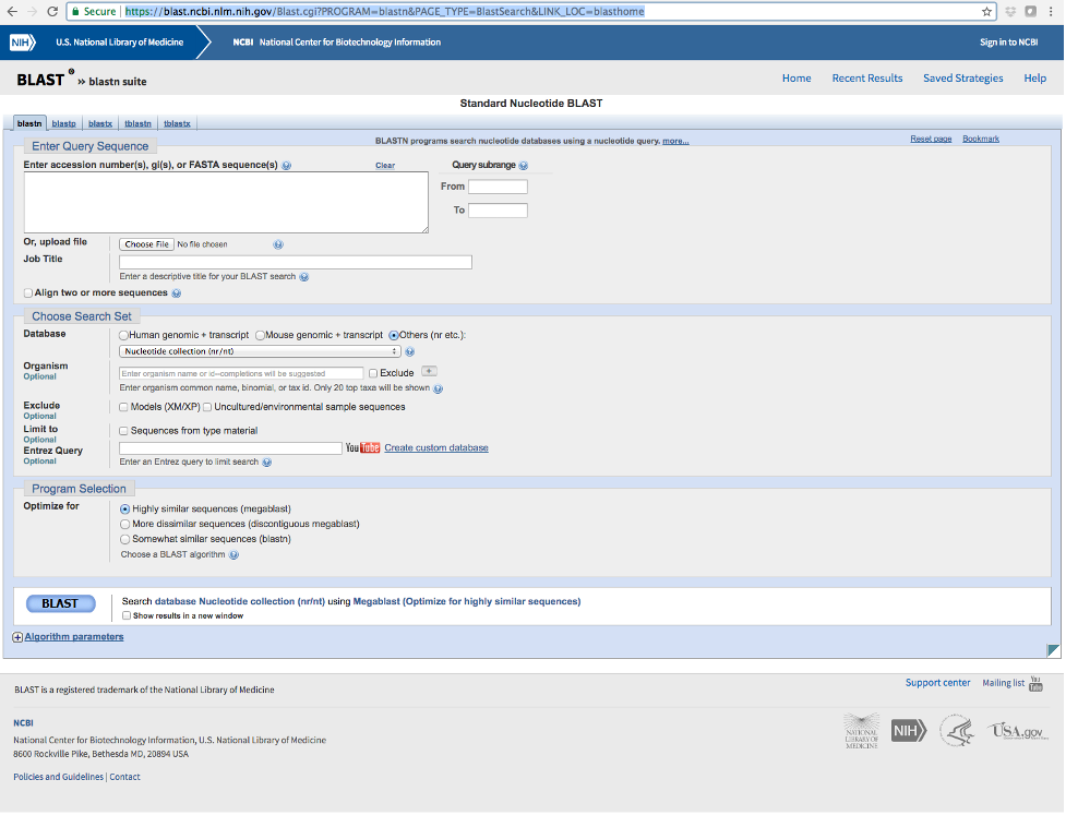
4. Make sure that ‘nucleotide collection’ is selected under Database and click the BLAST button.

 

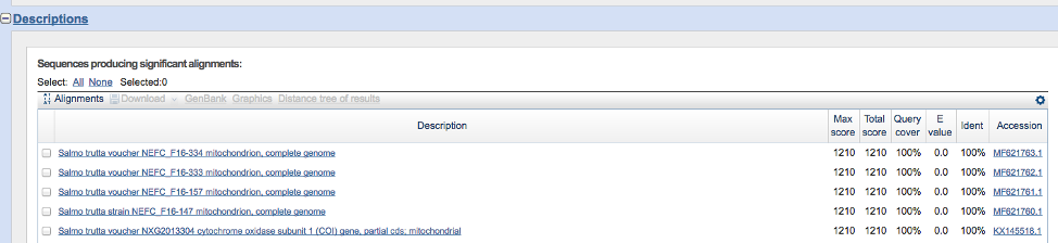
5. Scroll down until you see something resembling the image below. The ‘Query cover’ represents the proportion of your query sequence covered by the sequence match. For example, 100% of your query sequence aligns with the five samples in the figure below. The ‘Ident’ column indicates the sequence similarity between your query sequence and the matches. The five sequences below are 100% identical to your query sequence, suggesting that the species is Salmo trutta. Finally, the ‘E value’ column represents the number of matches expected simply by random chance (i.e. NOT due to homology/shared ancestry). Lower values indicate true matches due to homology.

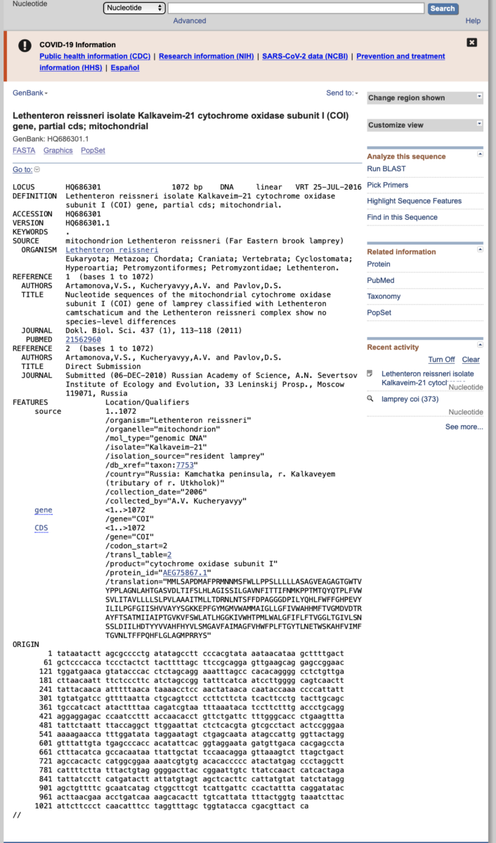
6. As we will be performing an evolutionary analysis of our fish sequences, we will need to obtain an outgroup sequence to root our phylogenetic tree. Outgroups are used to provide direction of evolutionary changes from ancestors to descendants. Outgroups should be from taxa closely related to the ingroup, but outside of the ingroup. Because we are working with fish species, a good outgroup might be from a mammal, bird, snake, or lizard. However, some students bring in shark tissue for analysis. In this case, using a tetrapod (amphibian, reptile, bird, or mammal) would not be appropriate because bony fish are more closely related to tetrapods than they are to cartilaginous fishes (sharks, skates, rays). Thus, for simplicity, we will use a lamprey as our outgroup. In NCBI, search for accession number HQ686301.1, which is a COI sequence from the Far Eastern Brook Lamprey, Lethenteron reissneri. Click on the accession to bring up a page like the one shown below. This page provides a ton of information about the sequence, such as the authors, publication, translation, etc. When ready, click the ‘Send to’ icon on the top right, send to file, and choose FASTA format. This will download the sequence in the same format as our fish sequences.

7. Next, import all the fish data and the outgroup sequence into Alivew to perform a multiple sequence alignment. Multiple sequence alignments are needed prior to evolutionary inference to determine homology among sequences. In essence, we need to make sure we are comparing apples to apples among our different species. Once all the data are imported into Aliview, click Align > realign everything. This will use the popular MUSCLE algorithm to align all your sequences. Once the data are aligned, export the alignment as a phylip

 

8. Our final objective is to perform a phylogenetic analysis of our sequences to determine evolutionary relationships. There are multiple optimality criteria used to build phylogenetic trees including maximum parsimony (MP), maximum likelihood (ML), and Bayesian inference (BI), the latter two of which are considered parametric methods because they rely on evolutionary models. Before we estimate a tree, we need to become a little familiar with what evolutionary models are.

 

Brief introduction to evolutionary models:

Evolutionary models are used to model changes in characters states (e.g. nucleotides) over the course of evolutionary time. For example, what is the probability of an adenine changing to a thymine versus a cytosine? These models can be used to estimate phylogenetic trees using maximum likelihood and Bayesian methods. So what exactly IS an evolutionary model? All evolutionary models have two components: base frequencies and nucleotide substitution rates. The simplest model, the Jukes-Cantor (JC) model, assumes that the four nucleotides occur at the same frequency in the alignment (25% each) and that the rate of nucleotide substitution is the same between any pair of nucleotides (e.g. A > C = A > T = G >T = C > T and so forth). The Felsenstein 81 (F81) model is the same as the JC model except it assumes unequal base frequencies (π_A ≠ π_C ≠ π_G ≠ π_T). The Kimura two parameter model (K2P) assumes equal base frequencies (π_A = π_C = π_G = π_T), but differentiates between the rate of transitions and transversions. Recall that a transition is between a purine to purine or between a pyrimidine to pyrimidine. In contrast, transversions are between a purine and pyrimidine. The HKY85 model expands the K2P model to include unequal base frequencies. The most parameter rich model is the General Time Reversible (GTR) model, which assumes unequal base frequencies and different substitution rates between every nucleotide pair. In general, more parameter rich models like HKY and GTR are needed for alignments with higher levels of polymorphism.

In addition to the classes of models discussed above, we can add two additional parameters to any model. The first accounts for invariable sites in a multiple sequence alignment, which we denote as I. The second parameter, gamma, controls for evolutionary rate variation across the alignment. For example, some regions of the alignment might be highly conserved, whereas other portions show many nucleotide substitutions. The amount of rate variation is controlled by a parameter alpha, with small values indicating high levels of rate variation across the alignment. These additional parameters (+I, +G) can be added to any of the models discussed above (e.g. HKY+I, GTR+I+G, JC+G, etc.).

It should be obvious by now that there are many potential models to be used to model the evolutionary process. So how do researchers know which model to use for a specific alignment? Fortunately, there are software packages available that can help select a model objectively. We will not go into model selection in further detail here as it is beyond the scope of the course.

 

Now that we are a little more comfortable with evolutionary models, let’s get back to our fish data. We just exported our multiple sequence alignment from Aliview as a phylip file. We will use the popular program IQ-TREE to estimate a phylogeny using the ML criterion. Navigate to www.iqtree.org to download the program to your computer. There are versions available for both Windows and Mac. IQ-TREE, and most phylogenetics packages, are command-line only and thus require some familiarity with the terminal. Fortunately, in IQ-TREE the commands are nearly identical between operating systems. One difference is that in Windows we use ‘\’ in our directory paths, whereas on a Mac we use ‘/’.

Once you have the program downloaded, place your phylip alignment file in the same directory as IQ-TREE. Next, we need to open up a terminal window. For Windows, click ‘Start’ and type “cmd”. This will open up a command line interface for your analysis. On a Mac, click the little magnifying glass on the upper right of your screen and type “terminal”.

Next, we need to change directory to where the program and data are. In both Windows and Mac we do this using the cd command. For example,

cd Documents/Programs/iqtree (for Mac)

cd Documents\Programs\qtree (for Windows)

We are now ready to run a ML phylogenetic analysis! IQ-TREE has many great options, but we will keep it basic here. Assuming you are on a Mac and in the iqtree directory, type the following command at the prompt:

./iqtree -s NameOfYourAlignment -B 10000 -alrt 1000 -o NameOfOutgroup

This command will perform multiple steps. First, IQ-TREE will search for the best nucleotide substitution model using ModelFinder. Next, it will use the best model to infer the ML phylogeny. Finally, it will assess node support using both the ultrafast bootstrap and SH-like approximate likelihood ratio tests. In general, ultrafast bootstrap values >95% and SH-aLRT > 80% indicate strong support for relationships. When the analysis finishes, you will see multiple output files in your working directory. Your instructor should take some time to go over these with you. The file ending with .treefile is your ML phylogeny.

Our next step is to view our fish phylogeny. Unfortunately, IQ-TREE is not the best place to view the tree. Instead, we will use the program FigTree (https://github.com/rambaut/figtree/releases). Download the relevant version for your system and open the program. Next, click ‘File/Open’ and navigate to your .treefile file. Click OK and your phylogeny should pop up. The first thing to do is root your phylogeny with the outgroup. Click on the branch leading to the lamprey and then click the ‘Reroot’ button in the menu. The next thing we want to do is show the support values for the nodes. Click on the box for ‘Branch Labels’ and then choose ‘label’. This will map on the aLRT/ultrafast bootstrap values on branches. Remember that values greater than 80% (aLRT) / 95% (bootstrap) indicate strong support. There are many other options worth exploring in FigTree. When ready, export your phylogeny as a pdf file.

 

Review questions

1. Paste your fish phylogeny in the space below and describe the phylogeny in your own words. Which species are sister taxa? Which are distantly related? Do your inferred relationships appear to agree with current taxonomy? If your samples included multiple species within a single genus (e.g. Salmo), was the genus monophyletic?

 

 

 

 

 

 

 

 

 

 

 

 

 

 

2. Discuss the utility of DNA barcoding for biodiversity assessment and conservation. How do you think the approach has advanced conservation efforts? How is DNA barcoding better than traditional morphological identification? What might be some limitations to barcoding?

 

 

 

 

 

 

 

3. As stated above, the COI gene is usually not an ideal marker for barcoding plants. Why might this be? What is different between the plant barcoding genes and COI?

 

 

 

 

 

 

4. In BLAST, what does the E-value indicate?

 

 

 

 

 

5. Why is the GTR+I+G model considered to be the most parameter rich? Describe the components of this model.

 

 

 

 

 

6. Why do we need to perform a multiple sequence alignment prior to phylogenetic inference?

 

 

 

 

 

7. Can you think of an example of when COI might not be a useful barcoding marker for animals? Explain your reasoning.

 

 

 

 

 

 

8. Compare and contrast homology, orthology and paralogy with respect to evolutionary inference. You may need to refer to your textbook for assistance.

 

 

 

 

 

 

9. Discuss how the statistical procedure of bootstrapping is used in phylogenetic inference. What is meant by a bootstrap replicate?

 

 

 

 

 

 

 

References

 

Arnold ML, Holman D, Zweifel S. 2017. Using molecular biology and bioinformatics to investigate the prevalence of mislabeled fish samples. The American Biology Teacher 79, 763-768.

 

Warner K, Timme W, Lowell B, Hirschfield M. 2013. Oceana study reveals seafood fraud nationwide. Retrieved from http://oceana.org/sites/default/files/reports/National_Seafood_Fraud_Testing_Results_Final.pdf.